Quantum Decoherence Visualization Documentation

Introduction

Quantum decoherence is a fundamental process in open quantum systems where quantum coherence is lost due to interaction with the environment. This simulation package provides tools to study decoherence effects on quantum tunneling and interference, using state-of-the-art numerical methods including the Lindblad master equation and quantum trajectories.

The simulation allows researchers and students to visualize how environmental interactions destroy quantum superpositions, leading from quantum to classical behavior. This is crucial for understanding quantum measurement, quantum computing, and the quantum-to-classical transition.

This package implements multiple decoherence models, supports various potential types, and provides real-time visualization through an interactive GUI, making it suitable for both research and educational purposes.

Features

Multiple Decoherence Models

Lindblad master equation, quantum trajectories, and stochastic unravelling methods

Flexible Potential Systems

Square barriers, double wells, Coulomb, Woods-Saxon, harmonic oscillator

Interactive GUI

Real-time parameter adjustment with live visualization of density matrices

Advanced Visualizations

Density matrix heatmaps, Wigner functions, purity/entropy tracking

Validation Tools

Built-in convergence tests and benchmark comparisons

Multiple Observables

Purity, von Neumann entropy, coherence, transmission probability

Physics Models

Lindblad Master Equation

The evolution of the density matrix with dissipative coupling is described by:

dρ/dt = -(i/ℏ)[H,ρ] + Σₖ γₖ(LₖρLₖ† - ½{Lₖ†Lₖ,ρ})

Key operators:

Dephasing: L = x̂ (position operator)
Relaxation: L = σ₋ (lowering operator)
Momentum diffusion: L = p̂ (momentum operator)

Quantum Trajectories

Monte Carlo wavefunction method for efficient large-scale simulations. Reduces memory cost from O(N²) to O(N) by evolving pure states stochastically rather than the full density matrix.

Supported Potentials

Square barrier: Tunneling through potential barrier
Double well: Quantum tunneling between wells
Coulomb: Bound states and scattering
Woods-Saxon: Nuclear physics potential
Harmonic oscillator: Parabolic confining potential

Decoherence Mechanisms

Dephasing: Random phase kicks destroy coherence
Energy relaxation: Spontaneous emission and absorption
Momentum diffusion: Collisional decoherence
Measurement backaction: Continuous weak measurement

Installation

System Requirements

Python: 3.8 or later
Required Packages: NumPy ≥1.21, SciPy ≥1.7, Matplotlib ≥3.4, Numba ≥0.56
Optional: ImageIO for GIF export
RAM: Minimum 4 GB (8 GB recommended for large grids)

Installation Steps

Ensure Python 3.8+ is installed
Download the simulation code package
Navigate to the project directory
Install dependencies:
pip install -r requirements.txt
Verify installation:
python -c "import numpy, scipy, matplotlib; print('All dependencies installed!')"

Quick Start

Option 1: Interactive GUI (Recommended)

                python gui.py
            

The GUI allows you to:

Adjust decoherence rate γ in real-time
Change potential parameters (barrier height, width)
Switch between Lindblad and quantum trajectories solvers
Visualize density matrices, purity, entropy, and coherence

Option 2: Simple Example

                python run_example.py
            

This will create a Gaussian wavepacket incident on a square barrier, evolve it with dephasing decoherence, and generate plots showing purity, entropy, and coherence evolution.

Option 3: Validation Notebooks

Run scientific validation examples:

                cd notebooks

                python basic_example.py          # Compare unitary vs decoherent evolution

                python trajectory_comparison.py  # Compare Lindblad vs trajectories

                python gamma_sweep.py            # Study decoherence effects on tunneling

Interactive GUI Controls

GUI Parameters

Grid Size: Number of spatial grid points (50-500, higher = more accurate but slower)
Potential Type: Square, double well, parabolic, Coulomb, or Woods-Saxon
V₀: Barrier height (0.1 - 10.0)
Barrier Width: Width of potential barrier (0.5 - 5.0)
Decoherence Rate γ: Strength of decoherence (0.0 - 2.0)
Solver Method: Lindblad (density matrix) or Quantum Trajectories
Time Parameters: Time step and final time

GUI Features

Real-time visualization of density matrices
Purity and entropy tracking over time
Coherence decay monitoring
Probability distribution display
Save figures and data export
Preset save/load functionality
GIF animation export (requires imageio)

Tip: Start with smaller grids (N=100-200) for faster testing, then increase for higher accuracy. Use quantum trajectories for N > 300 to reduce memory usage.

Python API Usage

Basic usage example:

                import numpy as np

                from hamiltonian import Hamiltonian1D, create_gaussian_wavepacket

                from lindblad import LindbladSolver, create_dephasing_operator

                from observables import purity, von_neumann_entropy, coherence

                # 1. Build system

                H = Hamiltonian1D(N=200, x_min=-10, x_max=10, 

                                      potential_type='square',

                                      potential_params={'V0': 1.5, 'width': 2.0})

                # 2. Create initial state

                psi0 = create_gaussian_wavepacket(H.x, x0=-5.0, sigma=1.0, k0=1.0)

                rho0 = np.outer(psi0, psi0.conj())

                # 3. Setup decoherence

                gamma = 0.1

                L = create_dephasing_operator(H.x, strength=1.0)

                solver = LindbladSolver(H.get_matrix(), [L], [gamma])

                # 4. Evolve

                rho_t, t = solver.evolve(rho0, t_final=5.0)

                # 5. Analyze

                P_t = purity(rho_t)  # Purity over time

                S = von_neumann_entropy(rho_t[-1])  # Final entropy

                C_t = coherence(rho_t)  # Coherence over time

                print(f"Final purity: {P_t[-1]:.4f}")

                print(f"Final entropy: {S:.4f}")

Observables and Metrics

Purity

Definition: P = Tr(ρ²)

P = 1: Pure state (no decoherence)
P < 1: Mixed state (decoherence occurred)
P → 1/N: Completely mixed (maximal decoherence)

Von Neumann Entropy

Definition: S = -Tr(ρ log ρ)

S = 0: Pure state, no uncertainty
S > 0: Mixed state, information loss
S increases: System loses coherence to environment

Coherence

Definition: C = Σᵢ≠ⱼ |ρᵢⱼ|

High C: Strong off-diagonal terms (quantum effects)
Low C: Diagonal density matrix (classical behavior)
Decoherence: C → 0 over time

Transmission Probability

Definition: T = ∫ᵦ |ψ(x)|² dx

Measures the tunneling probability through a potential barrier.

Wigner Function

Phase-space quasi-probability distribution providing complete quantum state information.

Example Results

Below is a visualization from the simulation using the animation preset demo parameters, which have been optimized to demonstrate dramatic decoherence effects. This example showcases how quantum coherence is lost over time, transitioning from a pure quantum state to a mixed state.

                Demo Preset Parameters:
                Grid Size: 180 points
Total Time: 5.0 (arbitrary units)
Time Steps: 150
Initial Wavepacket: x₀ = -6.0, σ = 1.2, k₀ = 1.5
Dephasing Rate γₓ: 0.6
Momentum Diffusion Rate γₚ: 0.2
Potential: Square barrier (V₀ = 1.0, width = 2.0)

            

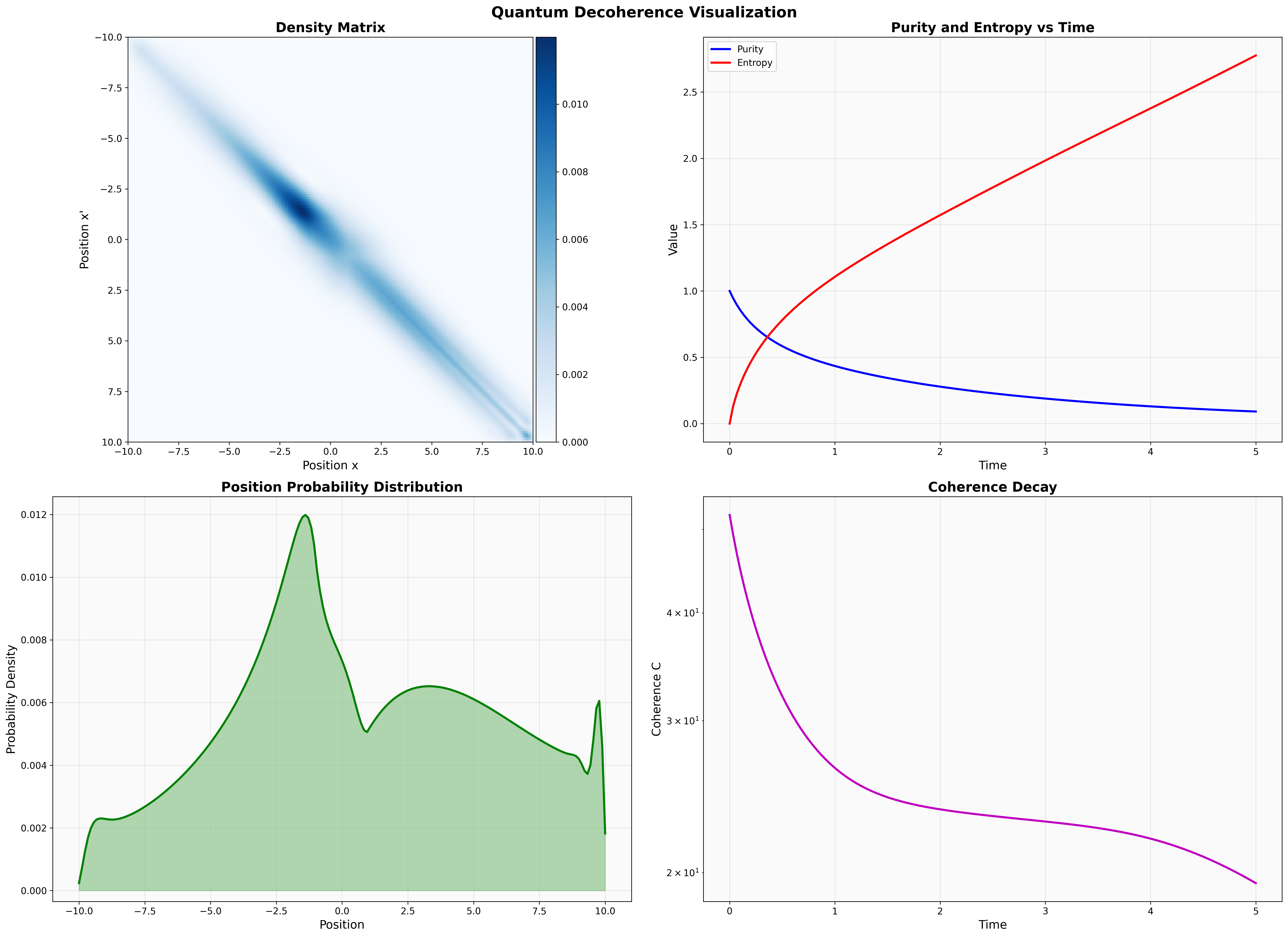
Quantum Decoherence Visualization - Demo Preset Results

Quantum Decoherence Visualization: Four-panel display showing density matrix evolution, purity/entropy dynamics, probability distribution, and coherence decay over time.

Key Observations

Density Matrix (Top-Left)

The heatmap reveals a prominent diagonal structure with off-diagonal coherence elements. The dark blue peak centered around (x=0, x'=0) shows strong position correlation, while the fading off-diagonal elements indicate loss of coherence as the system evolves.

Purity and Entropy (Top-Right)

The dramatic evolution demonstrates clear decoherence signatures:

Purity (Blue): Decreases from 1.0 (pure state) to ~0.25 (mixed state), showing the system transitions from quantum to classical behavior.
Entropy (Red): Increases from 0.0 to ~2.5, indicating increasing uncertainty and information loss to the environment.
The curves intersect around t ≈ 0.75, marking a critical transition point in the decoherence process.

Probability Distribution (Bottom-Left)

The multimodal distribution shows multiple probability peaks:

Primary peak at x ≈ -1.5 with maximum probability density ~0.012
Secondary peak at x ≈ 3.0 with density ~0.006
Sharp peak near x ≈ 9.5, indicating tunneling behavior

This complex distribution reflects the interplay between quantum tunneling and decoherence, where environmental interactions modify the probability landscape.

Coherence Decay (Bottom-Right)

The exponential-like decay curve (log scale) shows:

Rapid initial decay from ~40 to ~25 within the first time unit
Gradual asymptotic approach to ~20 by t = 5
Characteristic exponential decay pattern consistent with Lindblad dynamics

Physical Interpretation: This visualization demonstrates the quantum-to-classical transition, where environmental coupling (via dephasing and momentum diffusion) destroys quantum superpositions. The simultaneous decrease in purity and increase in entropy confirm that the system is losing quantum coherence and evolving toward a classically mixed state, as predicted by open quantum systems theory.

Validation

The code includes built-in validation checks:

Trace conservation: Tr(ρ) = 1 (density matrix normalization)
Positivity: All eigenvalues ≥ 0 (physical density matrix)
Purity bounds: 1/N ≤ P ≤ 1 (theoretical limits)
Benchmark comparisons: Validation against analytic limits
Convergence tests: For trajectory ensembles

Numerical Methods

Sparse matrices: Efficient Hamiltonian representation
Adaptive time stepping: RK45 ODE solver
Parallel trajectories: Multiprocessing for ensembles
Stability checks: Positivity preservation, trace conservation

Monitoring: Always monitor purity to ensure it stays ≤ 1 at all times. This serves as a positivity check for the density matrix evolution.

Citation

If you use this software in your research or educational materials, please cite:

BibTeX

                @software{uniphi_decoherence_2025,

                  author = {UniPhi Collective},

                  title = {Quantum Decoherence Visualization: A Python Simulation},

                  year = {2025},

                  note = {Lindblad master equation and quantum trajectories implementation}

                }

References

Schlosshauer, M. "Quantum decoherence and the measurement problem." Physics Reports 2008.
Breuer, H.-P. & Petruccione, F. The Theory of Open Quantum Systems. Oxford, 2002.

License

This simulation is released under the MIT License. You are free to use, modify, and distribute it for educational and research purposes. Please maintain attribution to the original authors.

Quantum Decoherence Visualization

Table of Contents