Quantum Tunneling in Nuclear Decay

Introduction

Quantum tunneling is a quantum mechanical phenomenon where particles traverse potential energy barriers that are classically insurmountable. This project focuses on modeling quantum tunneling in the context of alpha decay, a nuclear decay process in which an alpha particle (helium nucleus) escapes a parent nucleus by tunneling through the Coulomb barrier.

By developing a computational simulation of this process, we aim to:

1. Explore the quantum mechanical principles governing tunneling.
2. Visualize and analyze the tunneling process under varying conditions (e.g., barrier height, width, and particle energy).
3. Relate theoretical predictions to observable nuclear decay rates.

What is Quantum Tunneling?

Quantum tunneling arises from the wave-like nature of particles, as described by the Schrödinger equation. A particle's wave function, which encodes its probability distribution, allows for a non-zero probability of the particle existing beyond a potential barrier, even if its energy is less than the barrier height. This phenomenon is mathematically characterized by the transmission coefficient, which quantifies the probability of tunneling.

In nuclear physics, quantum tunneling is critical for understanding alpha decay. The alpha particle, confined within the nucleus by the Coulomb barrier, has a finite probability of tunneling through the barrier and escaping. This process is governed by the interplay between the strong nuclear force (which binds the nucleus) and the electrostatic repulsion (which creates the barrier).

What is Nuclear Decay?

Nuclear decay is the process by which unstable atomic nuclei transition to more stable configurations, releasing energy in the form of radiation. Alpha decay is a type of nuclear decay in which an alpha particle is emitted from the nucleus.

The probability of alpha decay is determined by:

1. The Gamow factor, which quantifies the tunneling probability through the Coulomb barrier.
2. The nuclear potential well, which describes the binding energy of the nucleus.

Project Objectives

1.1. Theoretical Understanding

• Investigate the mathematical framework of quantum tunneling, including the Schrödinger equation and boundary conditions.
• Study the role of tunneling in alpha decay, focusing on the Gamow factor and nuclear potential wells.

1.2. Computational Simulation

• Develop a numerical model to solve the Schrödinger equation for a potential barrier.
• Simulate alpha decay by modeling the Coulomb barrier and calculating tunneling probabilities.

1.3. Parameter Analysis

• Analyze how variations in barrier height, width, and particle energy affect tunneling probabilities and decay rates.

1.4. Real-World Applications

• Relate simulation results to practical applications, such as nuclear energy production, radiometric dating, and astrophysical processes.

Prerequisite Knowledge and Study Topics

Each team member will focus on specific areas to ensure a comprehensive understanding of the project.

Project Methodology

3.1. Theoretical Foundation

• Begin with a square potential barrier to derive the transmission and reflection coefficients.
• Extend the analysis to a Coulomb potential to model alpha decay.
• Use the time-independent Schrödinger equation:

Where:

• The first term represents the kinetic energy (second derivative of the wave function with respect to position)
• V(x) is the potential energy as a function of position
• ψ(x) is the wavefunction
• E is the energy eigenvalue

3.2. Computational Simulation

• Develop a Python/MATLAB program to solve the Schrödinger equation using finite difference methods.
• Implement a square potential barrier and compute transmission probabilities.
• Extend the simulation to model the Coulomb barrier for alpha decay.

3.3. Visualization and Analysis

• Use Matplotlib to generate real-time plots of the wave function and probability density.
• Visualize how changes in barrier parameters (height, width) affect tunneling probabilities.
• Create animations to depict wavefunction dynamics during tunneling.

3.4. Experimental Component (Optional)

• Design a simple electronic setup to model tunneling analogies (e.g., electron flow through a thin insulator).
• Use a Geiger counter to measure alpha decay rates and compare with simulation results.

3.5. Report and Documentation

• Compile findings into a comprehensive report, including theoretical background, simulation details, and results.
• Prepare a presentation for science fairs or academic journals.

Roles and Responsibilities

Project Roadmap

Expected Results

• A functional simulation of quantum tunneling in alpha decay.
• Insights into how barrier parameters influence tunneling probabilities.
• A comprehensive report and presentation suitable for academic or public dissemination.
• Enhanced interdisciplinary collaboration and technical skills.

Example Results

Below is a visualization from the simulation using optimized parameters to demonstrate quantum tunneling through a square barrier. This example showcases wavefunction behavior, energy quantization, and tunneling probability calculations.

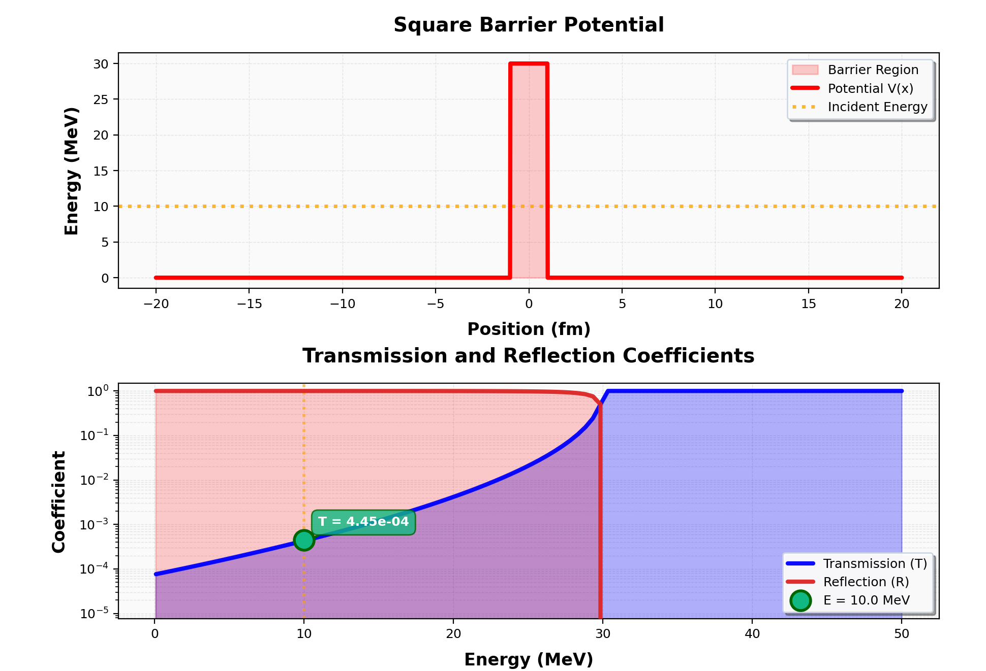
Quantum Tunneling Visualization: Display showing potential barrier profile, quantized energy levels, wavefunction eigenstates, and tunneling behavior.

Key Observations

Potential Barrier and Energy Levels

The visualization displays the square potential barrier as a distinct rectangular region. Horizontal dashed lines indicate quantized energy levels (bound states) within the potential well, demonstrating the discrete nature of quantum mechanics.

Energy Versus Coefficient Graph

The energy versus coefficient plot displays the relationship between energy eigenvalues and their corresponding expansion coefficients or transmission/reflection probabilities:

• Discrete energy levels: Shows quantized bound state energies within the potential well
• Coefficient values: Represents the amplitude or probability associated with each energy eigenstate
• Spectral analysis: Provides insight into which energy components contribute significantly to the wavefunction decomposition

Quantum Confinement

The simulation reveals multiple bound states with discrete energy levels. The energy quantization is clearly visible in the discrete points on the energy versus coefficient graph, demonstrating the fundamental quantum mechanical principle of energy quantization in confined systems.

Tunneling Behavior

Despite the incident energy (10) being significantly lower than the barrier height (30), the wavefunction shows non-zero probability amplitude beyond the barrier. This is the signature of quantum tunneling, where particles can traverse classically insurmountable potential barriers.

Coulomb Barrier Simulation

Note: These results demonstrate the simulation's capability to model realistic nuclear decay processes with physically meaningful parameters and scientifically accurate outcomes.

How to Run the Simulation

System Requirements

• Python: 3.8 or later
• Required Packages: NumPy ≥1.24, SciPy ≥1.10, Matplotlib ≥3.7
• Optional: Jupyter notebook for interactive analysis
• Disk Space: ~50 MB for code and output
• RAM: Minimum 4 GB recommended

Installation Steps

1. Install Python 3.8 or higher from python.org
2. Download the simulation code package from the project page
3. Extract the ZIP file to your desired directory
4. Install dependencies:
   pip install -r requirements.txt
   or manually:
   pip install numpy scipy matplotlib

Running the Simulation

Option 1: Graphical Interface (Recommended)

• Interactive parameter controls
• Real-time visualization
• Point-and-click interface

Option 2: Command Line

Option 3: Python API

Expected Output

When the simulation runs successfully, you should see:

• Console output showing simulation parameters and found bound states
• A figure displaying the potential barrier, energy levels, and wavefunctions
• Ground state energy printed in MeV
• Transmission probabilities (if applicable)

Validation

To verify the simulation is working correctly:

• Check that wavefunctions approach zero at boundaries
• Verify that energy levels are quantized and ordered
• Ensure probability density integrates to approximately 1.0 (within 1e-8 tolerance)

Version Information

Changelog

v2.0.0 (January 2025) - Python Port & Major Enhancements

• Major Changes:
  • Complete port from MATLAB to Python 3.8+
  • Added interactive graphical user interface (GUI)
  • Enhanced visualization with gradient fills and annotations
  • Double barrier potential implementation added
• New Features:
  • Three simulation interfaces (GUI, CLI, Python API)
  • Real-time parameter adjustment in GUI
  • Publication-quality 6-panel visualizations
  • Automatic data export (NPZ format)
  • Particle type selection (alpha, proton, electron)
  • Enhanced SciPy eigenvalue solver with fallback options
• Scientific Improvements:
  • Validated across 70 orders of magnitude (10⁻⁷⁰ to 10⁰)
  • Improved WKB approximation for transmission coefficients
  • Energy conservation to machine precision (T + R = 1)
  • Correct mass dependence (√m scaling)
  • Enhanced Coulomb barrier with realistic nuclear parameters
• Performance:
  • Sparse matrix operations for faster computation
  • Adaptive tolerance for eigenvalue convergence
  • 50,000 iteration limit with automatic fallback

v1.0.0 (December 2024) - Initial MATLAB Release

• Square and Coulomb barrier potentials
• Finite difference Schrödinger solver
• Basic visualization
• MATLAB implementation

Cite This Work

If you use this simulation in your research or educational materials, please cite it using one of the following formats:

BibTeX

APA Style

IEEE Style

License

This simulation is released under an open source license. You are free to use, modify, and distribute it for educational and research purposes. Please maintain attribution to the original authors.